Bayesian Power Analysis in R – Ben R Woodard’s Blog

How can you tell if the two groups are different, I mean different enough to make a decision?

Setup

I need to run a test that will have a good chance of getting results. How long should I run it for?

# install.packages("rstanarm")  # if needed
library(rstanarm)

Loading required package: Rcpp

This is rstanarm version 2.32.2

- See https://mc-stan.org/rstanarm/articles/priors for changes to default priors!

- Default priors may change, so it's safest to specify priors, even if equivalent to the defaults.

- For execution on a local, multicore CPU with excess RAM we recommend calling

  options(mc.cores = parallel::detectCores())

library(tidyverse)

── Attaching core tidyverse packages ──────────────────────── tidyverse 2.0.0 ──
✔ dplyr     1.1.4     ✔ readr     2.1.5
✔ forcats   1.0.0     ✔ stringr   1.5.2
✔ ggplot2   4.0.0     ✔ tibble    3.3.0
✔ lubridate 1.9.4     ✔ tidyr     1.3.1
✔ purrr     1.1.0

── Conflicts ────────────────────────────────────────── tidyverse_conflicts() ──
✖ dplyr::filter() masks stats::filter()
✖ dplyr::lag()    masks stats::lag()
ℹ Use the conflicted package (<http://conflicted.r-lib.org/>) to force all conflicts to become errors

# library(ggplot2)  # optional, for plotting

set.seed(1234)

2. Data generator: simulate an A/B test for a given number of days

Key Terms:

baseline_p = control conversion rate
lift = relative lift in treatment (e.g. 0.1 = +10% relative)
visitors_per_day = total visitors per day (split 50/50)

simulate_ab_binomial_days <- function(
  days,
  visitors_per_day = 5000,
  baseline_p       = 0.05,
  lift             = 0.10   # 10% relative lift
) {
  days = 14
  n_control_per_day  <- floor(visitors_per_day / 2)
  n_treat_per_day    <- visitors_per_day - n_control_per_day
  
  n_control <- n_control_per_day * days
  n_treat   <- n_treat_per_day   * days
  
  p_control <- baseline_p
  p_treat   <- baseline_p * (1 + lift)
  
  y_control <- rbinom(1, n_control, p_control)
  y_treat   <- rbinom(1, n_treat,   p_treat)
  
  data.frame(
    group    = factor(c("Control", "Treatment"),
                      levels = c("Control", "Treatment")),
    successes = c(y_control, y_treat),
    failures  = c(n_control - y_control,
                  n_treat   - y_treat)
  )
}

3. Fit Bayesian logistic model in rstanarm

We use a simple binomial regression: cbind(successes, failures) ~ group.

fit_bayes_ab <- function(dat,
                         iter   = 1000,
                         chains = 2) {
  stan_glm(
    cbind(successes, failures) ~ group,
    data   = dat,
    family = binomial(),
    prior           = normal(0, 1, autoscale = TRUE),
    prior_intercept = normal(0, 5, autoscale = TRUE),
    chains = chains,
    iter   = iter,
    cores  = 1,   # keep it simple & robust
    refresh = 0
  )
}

4. Bayesian decision rule: “Is treatment better?”

We use the posterior difference in conversion rates (not just the log-odds).

compute_decision <- function(fit,
                             prob_threshold = 0.95) {
  nd <- data.frame(
    group = factor(c("Control", "Treatment"),
                   levels = c("Control", "Treatment"))
  )
  
  # Posterior predicted conversion rate for each group
  pred <- posterior_epred(fit,
                            newdata  = nd)  # on probability scale
  
  # pred: draws x 2 (Control, Treatment)
  diff_draws <- pred[, 2] - pred[, 1]        # Treatment - Control
  
  post_prob <- mean(diff_draws > 0)          # P(Treatment > Control)
  list(
    posterior_prob = post_prob,
    success        = post_prob >= prob_threshold
  )
}

5. Simulation-based “power” for a given duration

For a given number of days, we:

Simulate many fake tests.

Fit the Bayesian model each time.

Apply the decision rule.

Estimate how often we’d “declare a win”.

That frequency is your Bayesian power for that duration.

bayes_power_for_days <- function(
  days,
  visitors_per_day = 5000,
  baseline_p       = 0.05,
  lift             = 0.10,
  sims             = 100,    # bump up later (e.g. 500–1000)
  prob_threshold   = 0.95,
  iter             = 1000,
  chains           = 2
) {
  results <- map_dfr(1:sims, function(i) {
    dat <- simulate_ab_binomial_days(
      days            = days,
      visitors_per_day = visitors_per_day,
      baseline_p      = baseline_p,
      lift            = lift
    )
    
    fit <- fit_bayes_ab(dat, iter = iter, chains = chains)
    dec <- compute_decision(fit, prob_threshold = prob_threshold)
    
    tibble(
      sim            = i,
      posterior_prob = dec$posterior_prob,
      success        = dec$success
    )
  })
  
  power_est <- mean(results$success)
  mean_prob <- mean(results$posterior_prob)
  
  list(
    days                = days,
    power_estimate      = power_est,
    mean_posterior_prob = mean_prob,
    results             = results
  )
}

6. Estimate required duration: run over a grid of days

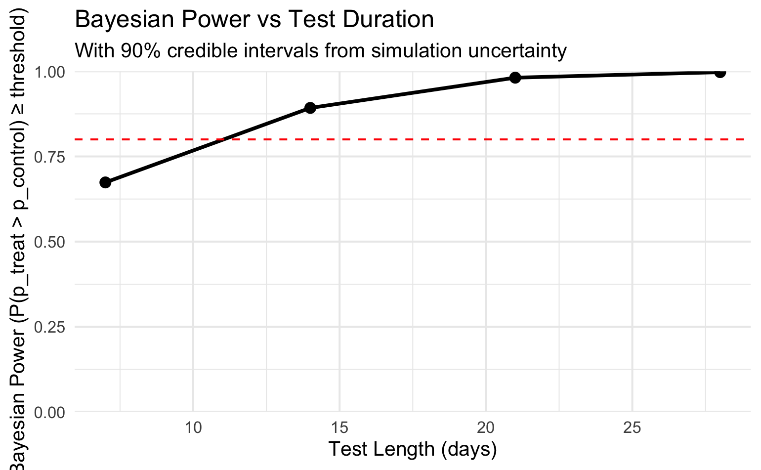
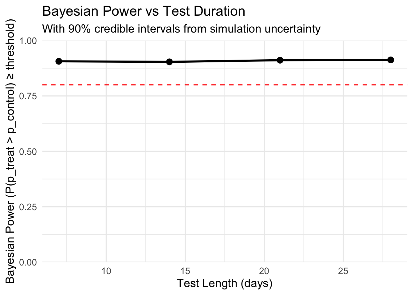
Now we check, say, 7, 10, 14, 21, 28 days and see where power crosses your target (e.g. 0.8).

days_grid <- c(7, 14, 21, 28)

power_grid <- map_dfr(days_grid, function(d) {
  
  res <- bayes_power_for_days(
    days             = d,
    visitors_per_day = 5000,
    baseline_p       = 0.05,
    lift             = 0.10,   # 10% relative effect
    sims             = 800,    # increase to 500+ for production
    prob_threshold   = 0.95
  )
  
  # Compute credible interval of the success indicator (power)
  ci_lower <- quantile(res$results$posterior_prob, 0.05)
  ci_upper <- quantile(res$results$posterior_prob, 0.95)
  
  tibble(
    days                = d,
    power_estimate      = res$power_estimate,
    mean_prob           = mean(res$results$posterior_prob),
    ci_lower            = ci_lower,
    ci_upper            = ci_upper
  )
})

power_grid

# A tibble: 4 × 5
   days power_estimate mean_prob ci_lower ci_upper
  <dbl>          <dbl>     <dbl>    <dbl>    <dbl>
1     7          0.906     0.985    0.920        1
2    14          0.904     0.980    0.897        1
3    21          0.911     0.981    0.903        1
4    28          0.912     0.981    0.904        1

Then you’d say something like:

“To detect a 10% lift with P(treatment > control | data) ≥ 0.95 about 80–90% of the time, I need around 14–21 days at 5k visitors/day and 5% baseline.”

ggplot(power_grid, aes(x = days, y = power_estimate)) +
  geom_line(size = 1.2) +
  geom_point(size = 3) +
  geom_hline(yintercept = 0.8, linetype = "dashed", color = "red") +
  scale_y_continuous(limits = c(0, 1), expand = c(0, 0)) +
  labs(
    title = "Bayesian Power vs Test Duration",
    subtitle = "With 90% credible intervals from simulation uncertainty",
    x = "Test Length (days)",
    y = "Bayesian Power (P(p_treat > p_control) ≥ threshold)"
  ) +
  theme_minimal(base_size = 14)

Warning: Using `size` aesthetic for lines was deprecated in ggplot2 3.4.0.
ℹ Please use `linewidth` instead.

Conclusion

Using a Bayesian approach to power analysis brings many more capabilities that the Frequentist approach does not. Some of these differences are more beneficial than others but overall, utilizing the Bayesian approach to power analysis is a great option.

Capability	Frequentist	Bayesian
Connect power to an actual business decision	❌	✅
Incorporate prior information	❌	✅
Use a distribution of plausible effect sizes	❌	✅
Simulate adaptive/sequential stopping	❌ (hard)	✅ (easy & valid)
Directly answer “probability treatment is better”	❌	✅
Model realistic data-generating processes	Limited	Excellent
Handle hierarchical/geo experiments	Hard	Natural
Provide interpretable outputs	❌	✅