The workhorse of all data science work is the basic linear regression model. It has the capability to change the direction of a business like a rudder on a boat but like a rudder, it is often overlooked by most practicioners until other more ‘advanced’ tactics are tried.
Here is an example of a basic bayesian linear regression model in R and stan.
Simulating the data is pretty straight forward.
set.seed (123 )<- 100 <- rnorm (N, 0 , 1 )<- 2.5 <- 0.8 <- 1.0 <- alpha_true + beta_true * x + rnorm (N, 0 , sigma_true)<- data.frame (x, y)head (df)
            x        y
1 -0.56047565 1.341213
2 -0.23017749 2.572742
3  1.55870831 3.500275
4  0.07050839 2.208864
5  0.12928774 1.651812
6  1.71506499 3.827024
Now that we have the data we want to create a linear regression model that shows the results of
<- lm (y ~ x, data = df)summary (lm_fit)
Call:
lm(formula = y ~ x, data = df)

Residuals:
    Min      1Q  Median      3Q     Max
-1.9073 -0.6835 -0.0875  0.5806  3.2904

Coefficients:
            Estimate Std. Error t value Pr(>|t|)
(Intercept)  2.39720    0.09755  24.574  < 2e-16 ***
x            0.74753    0.10688   6.994  3.3e-10 ***
---
Signif. codes:  0 '***' 0.001 '**' 0.01 '*' 0.05 '.' 0.1 ' ' 1

Residual standard error: 0.9707 on 98 degrees of freedom
Multiple R-squared:  0.333, Adjusted R-squared:  0.3262
F-statistic: 48.92 on 1 and 98 DF,  p-value: 3.304e-10
Key parts of summary(lm_fit):
Estimate: point estimates of intercept and slope
Std. Error: estimated standard error of each coefficient
t value, Pr(>|t|): classical hypothesis test for each coefficient
Residual standard error: estimate of σ
Multiple R-squared: variance explained
                2.5 %    97.5 %
(Intercept) 2.2036098 2.5907841
x           0.5354312 0.9596255
Interpretation (frequentist):
If we repeated this estimation procedure infinitely many times, 95% of the constructed intervals would contain the true parameter.
(Contrast: in Bayesian, you’d say “there’s a 95% probability the parameter lies in this interval, given data + priors.”)
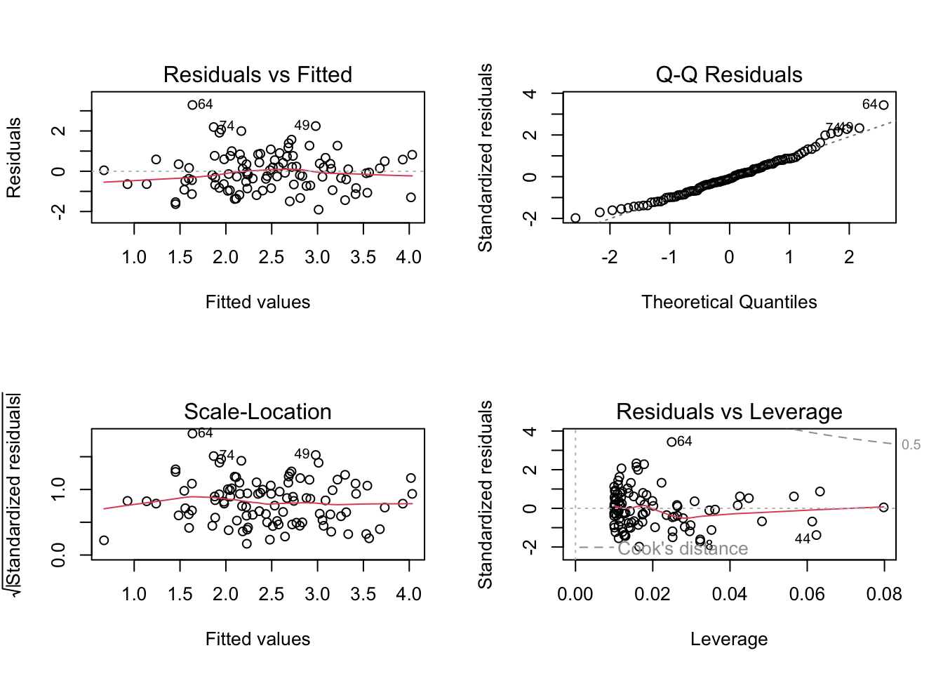
Basic Diagnostic Plots
par (mfrow = c (2 , 2 ))plot (lm_fit)
You get:
Residuals vs Fitted (linearity, homoskedasticity)
Normal Q-Q (normality of residuals)
Scale-Location
Residuals vs Leverage (influence)
Predictions with confidence & prediction intervals
<- data.frame (x = seq (- 2 , 2 , length.out = 30 ))# Confidence interval for the *mean* response <- predict (lm_fit, newdata = new, interval = "confidence" , level = 0.95 )# Prediction interval for a *new* observation <- predict (lm_fit, newdata = new, interval = "prediction" , level = 0.95 )head (pred_conf)
        fit       lwr      upr
1 0.9021402 0.4187310 1.385549
2 1.0052475 0.5485212 1.461974
3 1.1083549 0.6779769 1.538733
4 1.2114623 0.8070330 1.615892
5 1.3145696 0.9356071 1.693532
6 1.4176770 1.0635953 1.771759
        fit        lwr      upr
1 0.9021402 -1.0839403 2.888221
2 1.0052475 -0.9745075 2.985003
3 1.1083549 -0.8654881 3.082198
4 1.2114623 -0.7568858 3.179810
5 1.3145696 -0.6487041 3.277843
6 1.4176770 -0.5409462 3.376300
“confidence” = uncertainty about E[y | x]
“prediction” = uncertainty about a new y at that x (includes residual noise, so wider)
library (ggplot2)<- cbind (new, as.data.frame (pred_conf))names (pred_df) <- c ("x" , "fit" , "lwr" , "upr" )# ggplot(df, aes(x, y)) + # geom_point(alpha = 0.7) + # geom_line(data = pred_df, aes(x, fit)) + # geom_ribbon( # data = pred_df, # aes(x = x, ymin = lwr, ymax = upr), # alpha = 0.2 # ) + # labs( # title = "Frequentist Linear Regression (lm)", # subtitle = "Fitted line with 95% confidence band for mean response" # )
Quick contrast with your Bayesian version Using the same simulated data:
Frequentist (lm):
Coefficients: point estimates + SE
95% CIs: coverage interpretation over repeated samples
p-values: H₀ tests (β = 0, etc.)
Bayesian (stan_glm):
Coefficients: full posterior distributions
95% intervals: “credible intervals” (probability statements given model + priors)
No p-values; you might instead look at Pr(β > 0) or posterior density.

